Friday, December 30, 2011
Tuesday, December 20, 2011
Researchers Turn an Ordinary Canon 5D Into a Hyperspectral Camera
Hyperspectral imaging goes beyond what the human eye can see, collecting information from across the electromagnetic spectrum for use in analyzing a particular object or location (seeing if certain mineral deposits are present, for example). The specialized equipment doesn't run cheap, but researchers at the Vienna University of Technology have been able to turn an ordinary consumer DSLR camera into a full-fledged computed tomography image spectrometer.

Starting with a Canon EOS 5D, the team added a frankenlens made of PVC pipe and a diffraction gel combined with a 50mm, 14-40mm, and a +10 diopter macro lens. They were then able to mathematically reconstruct the full range of spectra from the data captured by the camera's imaging sensor, achieving performance comparable to that of commercial imagers: a resolution of 4.89nm in a hyperspectral configuration of 120 x 120 pixels. The downside is exposure time, with the DSLR requiring several seconds to capture the data, while tailor-made devices need mere milliseconds. The team admits that the current system is on the "low-end" of what is possible, but they already have their sights set on a direct-mount version, which will increase the aperture and lower the necessary exposure time — all while costing under $1,000.
via Technische Universtat Wien
Tuesday, December 6, 2011

Monday, December 5, 2011


Saturday, December 3, 2011
VP8 vs H.264
First, the conclusions for the lazy:
- VP8 is very similar to H.264, but it does not have better quality, nor is it faster.
- In the face of such striking similarities, the burden of proving VP8 being patent-free is still on Google.
- The VP8 spec is not complete or final in any way, so it might take time to integerate this codec into hardware devices.
- and lastly, having no hardware-accelerated support in existing smartphones/mobile-devices for decoding VP8 makes it very CPU and battery intensive.
One thing good about VP8: it does away with interlacing. Who needs it today, anyway? But VP8 lacks B-frames. What? B-frames can give 10-20% (or more) compression benefit for minimal speed cost.
References:
- The first in-depth technical analysis of VP8, by a third-year college student named Jason Garrett-Glaser, who works on the open source x264 project, a free software library for encoding video in H.264.
- Steve Jobs backed his claim than VP8 is not ready for prime time by the URL to Garrett-Glaser's blog post.
- VP8: a retrospective, another comment by Dark Shikari
- Moscow State University report on H.264 compared to other codecs.
- MSU Seventh MPEG-4 AVC/H.264 Video Codecs Comparison
Friday, December 2, 2011
How NOT to Upgrade Linux Mint from Katya to Lisa
The way to upgrade an Ubuntu-based distro (copied from a lucky person who got is working):
- Open a terminal and run 'sudo bash' to get a root terminal
- Using a text editor (as root), replace the contents of /etc/apt/sources.list with the following sources list:
deb http://packages.linuxmint.com/ lisa main upstream import backport
deb http://archive.ubuntu.com/ubuntu/ oneiric main restricted universe multiverse
deb http://archive.ubuntu.com/ubuntu/ oneiric-updates main restricted universe multiverse
deb http://security.ubuntu.com/ubuntu/ oneiric-security main restricted universe multiverse
deb http://archive.canonical.com/ubuntu/ oneiric partner
deb http://packages.medibuntu.org/ oneiric free non-free - Run 'apt-get update'
- Run 'apt-get dist-upgrade'
- Follow the instructions issued, don't worry about overwriting configuration files dpkg will keep a copy in the same directory with the string ".dpkg-old" appended to the filename
- Run 'apt-get upgrade'
- Reboot
Theoretically, the steps above should be sufficient for Ubuntu upgrading. But Linux Mint discourages in situ upgrades. The recommended way is to back up all personal files and reinstall with new ISO.
I should know. The steps above left me with a system that doesn't allow me to login. Arrgh! I'm beginning to like Fedora more and more already.
Thursday, December 1, 2011
ffmpeg sample use collection
Caveat: may not work in all cases
Very important, add "-threads 0" to every ffmpeg invocation to use all available cores.
- http://juliensimon.blogspot.com/2008/12/howto-quick-reference-on-audio-video.html
- http://dev.heywatch.com/doc/coreapi/x264_presets.html
Very important, add "-threads 0" to every ffmpeg invocation to use all available cores.
Tuesday, November 29, 2011
ffmpeg install with libx264 (h264) on Fedora
The information for this is VERY very sparse, so here is a summary of what I have found.
Get all the fancy codecs
Install libx264
Get the libx264 package from http://www.videolan.org/developers/x264.html.
The link to the actual file is ftp://ftp.videolan.org/pub/x264/snapshots/last_x264.tar.bz2
Download it, then..
Install ffmpeg
Just use your browser. From http://ffmpeg.org/download.html find the latest stable release, which is currently http://ffmpeg.org/releases/ffmpeg-0.8.7.tar.bz2. Download it, then...
ffmpeg is now installed with libx264 (h264).
Courtesy: http://www.saiweb.co.uk/linux/ffmpeg-install-with-libx264-h264
It works! I'm no longer getting Unknown encoder 'libx264' message.
Use ffmpeg
For example, convert a Flash video compressed using VP8 codec to H264. Am wondering which codec produces a smaller file.
Wait, and shazam! A smaller file should be produced. But you may get this message:
This error usually comes when ldconfig does not know where to search for the libraries, so, in order to help it out, on Fedora do the following:
Add another file: custom-libs.conf
Inside, put :
save, then do
et voila again!!!
Get all the fancy codecs
# yum -y install libmatroska-devel libmkv-devel mkvtoolnix-gui ogmrip themonospot-plugin-mkv themonospot amrnb-tools amrnb-devel amrnb amrwb-tools amrwb-devel amrwb bzip2-devel bzip2-libs bzip2 libdc1394-tools libdc1394-devel libdc1394 dirac-libs dirac-devel dirac faac-devel faac faad2-libs.x86_64 faad2-devel faad2 gsm-tools gsm-devel gsm lame-libs lame-devel lame twolame-libs twolame-devel twolame openjpeg-libs openjpeg-devel openjpeg ImageMagick schroedinger-devel schroedinger speex-tools speex-devel speex libtheora-devel theora-tools byzanz istanbul libtheora libvorbis-devel vorbisgain liboggz-devel libfishsound vorbis-tools x264-libs x264-devel x264 h264enc imlib2-devel libvdpau-devel opencore-amr-devel SDL-devel texi2html xvidcore-devel yasm
Install libx264
Get the libx264 package from http://www.videolan.org/developers/x264.html.
The link to the actual file is ftp://ftp.videolan.org/pub/x264/snapshots/last_x264.tar.bz2
Download it, then..
# cd ~/Downloads/
# tar -xjvf last_x264.tar.bz2
# cd last_x264
# ./configure --enable-shared
# make
# make install
# ldconfig
Install ffmpeg
Just use your browser. From http://ffmpeg.org/download.html find the latest stable release, which is currently http://ffmpeg.org/releases/ffmpeg-0.8.7.tar.bz2. Download it, then...
# cd ~/Downloads
# tar xvfj ffmpeg-0.8.7.tar.bz2
# cd ffmpeg-0.8.7
# ./configure --enable-libx264 --enable-gpl --enable-shared
# make
# make install
ffmpeg is now installed with libx264 (h264).
Courtesy: http://www.saiweb.co.uk/linux/ffmpeg-install-with-libx264-h264
It works! I'm no longer getting Unknown encoder 'libx264' message.
Use ffmpeg
For example, convert a Flash video compressed using VP8 codec to H264. Am wondering which codec produces a smaller file.
# ffmpeg -i aflashfile.flv -vcodec libx264 convertedfile.mp4
Wait, and shazam! A smaller file should be produced. But you may get this message:
error while loading shared libraries: libavdevice.so.52: cannot open shared object file: No such file or directory
This error usually comes when ldconfig does not know where to search for the libraries, so, in order to help it out, on Fedora do the following:
# cd /etc/ld.so.conf.d
Add another file: custom-libs.conf
Inside, put :
/usr/local/lib
save, then do
# ldconfig
et voila again!!!
Monday, November 21, 2011
Syntax Highlighting with Alex Gorbatchev's SyntaxHighliter 3.0
After struggling with it for a while, I managed to get Alex Gorbatchev's SyntaxHighlighter to work.
The steps are:
1) Go to Blogspot's Design -> Edit Html page.
2) Find the </head> tag. Just before it, past the following code:
Replace all occurences of <version> with current.
3) Find the </body> tag. Just before it, past the following code:
4) Start adding code snippets with
<pre> tags. Example:
5) The result of the above code would be:-
The steps are:
1) Go to Blogspot's Design -> Edit Html page.
2) Find the </head> tag. Just before it, past the following code:
Replace all occurences of <version> with current.
3) Find the </body> tag. Just before it, past the following code:
4) Start adding code snippets with
<pre> tags. Example:
alert('This is an example!');
5) The result of the above code would be:-
alert('This is an example!');
Friday, November 18, 2011

Wednesday, November 16, 2011
Linux Mint lebih popular dari Ubuntu
Mengikut perangkaan lelaman DistroWatch, Linux Mint telah mengatasi kepopularan Ubuntu. Ketua Linux Mint, Clint Lefevre, mengakui Linux Mint meningkat 40% pada bulan lepas, dan kebanyakan pengguna berasal dari Ubuntu. Di lelaman Linux Mint, dinyatakan pengguna Linux Mint sekitar 1/3 pengguna Ubuntu, menjadikannya OS keempat paling popular selepas Windows, Mac OS X dan Ubuntu.
Oh ya, saya dah menggunakannya selama dua minggu, sebelum menyedari ia begitu popular!! Saya memilih Linux Mint kerana ia tidak mempunyai 'buntu' dalam namanya....
Oh ya, saya dah menggunakannya selama dua minggu, sebelum menyedari ia begitu popular!! Saya memilih Linux Mint kerana ia tidak mempunyai 'buntu' dalam namanya....
Thursday, November 10, 2011
SURF - Speeded Up Robust Features
SURF stands for Speeded-Up Robust Features. It is inspired by SIFT, and is intended for applications that requires speed but does not require the precision of SIFT. SURF generates 64 features compared to SIFT which generates 128 features.
- SURF notes by Yet Another Blogger here.
Wednesday, November 9, 2011
FLANN Overview
Fast Library Approximate Nearest Neighbor (FLANN) algorithm was proposed by Marius Muja and David G. Lowe.
FLANN is a way to solve the nearest neighbor search (NNS), also known as proximity search, similarity search or closest point search, is an optimization problem for finding closest points in metric spaces. Donald Knuth in vol. 3 of The Art of Computer Programming (1973) called it the post-office problem, referring to an application of assigning to a residence the nearest post office.
A simple way to solve the nearest neighbor problem is by the k-NN algorithm, but k-NN will not work in very complex problems such as matching SIFT or SURF keypoints. An intermediate solution is to use KD-trees.
Tuesday, November 8, 2011
atan2 overview
The atan2 function computes the principal value of the arc tangent of y / x, using the signs of both arguments to determine the quadrant of the return value. It produces correct results even when the resulting angle is near π/2 or -π/2 (or x near 0).
The atan2 function is used mostly to convert from rectangular (x,y) to polar (r, θ) coordinates that must satisfy x = r cos(θ) and y = r sin (θ). In general, conversions to polar coordinates should be computed thus
The atan2 function is used mostly to convert from rectangular (x,y) to polar (r, θ) coordinates that must satisfy x = r cos(θ) and y = r sin (θ). In general, conversions to polar coordinates should be computed thus


- atan2 ( ±0, -0) returns ± π.
- atan2 ( ±0, +0 ) returns ±0.
- atan2 ( ±0, x ) returns ±π for x < 0.
- atan2 ( ±0 , x ) returns ±0 for x > 0.
- atan2 ( ±0 ) returns -π/2 for y > 0.
- atan2 ( ±y, -∞ ) returns ±π for finite y > 0.
- atan2 ( ±y, +∞ ) returns ±0 for finite y > 0.
- atan2 ( ±∞, +x ) returns ±π/2 for finite x.
- atan2 ( ±∞, -∞ ) returns ±3π/4.
- atan2 ( ±∞, +∞ ) returns ±π/4.
Thursday, November 3, 2011

GCC 4.6 breaks SystemC
When upgrading to Ubuntu 11.10, SystemC programs won't work anymore.
Update your makefiles to include the -fpermissive flag, like so:
You may need to recompile the SystemC library, which case the flag must be added to the configure command:
By giving the syntax above, I also managed to get SystemC running in Fedora. Goodbye Ubuntu!
Update your makefiles to include the -fpermissive flag, like so:
SYSTEMC=/usr/local/systemc
LDFLAGS= -L$(SYSTEMC)/lib-linux -lsystemc
CXXFLAGS=-Wno-deprecated -I$(SYSTEMC)/include -fpermissive

all:
 g++ $(CXXFLAGS) *.cpp $(LDFLAGS)
 ./a.out
You may need to recompile the SystemC library, which case the flag must be added to the configure command:
$ sudo ../configure --prefix=/usr/local/systemc CPPFLAGS=-fpermissive
By giving the syntax above, I also managed to get SystemC running in Fedora. Goodbye Ubuntu!
Wednesday, November 2, 2011
Removing unneeded Fedora kernels
Install the yum-utils package from Fedora Extras (
then do
By default package-cleanup keeps the last 2 kernels on the systems, just in the case the latest blows up.
# yum install yum-utils
then do
# package-cleanup --oldkernels"
By default package-cleanup keeps the last 2 kernels on the systems, just in the case the latest blows up.
Thursday, October 27, 2011
Another square root clipping
This time from Paul Hsieh
Begin quoted text
√(Δx2+Δy2) < d is equivalent to Δx2+Δy2 < d2, if d ≥ 0
End quoted text
Reference: http://www.azillionmonkeys.com/qed/sqroot.html
Begin quoted text
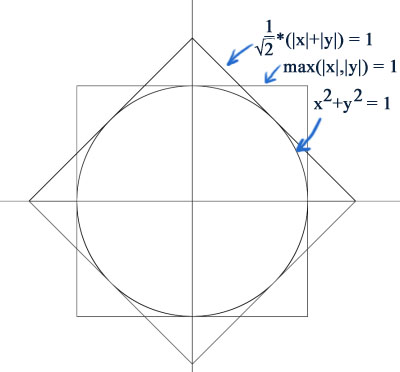
A common application in computer graphics, is to work out the distance between two points as √(Δx2+Δy2). However, for performance reasons, the square root operation is a killer, and often, very crude approximations are acceptable. So we examine the metrics (1 / √2)*(|x|+|y|), and max(|x|,|y|):
Notice the octagonal intersection of the area covered by these metrics, that very tightly fits around the ordinary distance metric. The metric that corresponds to this, therefore is simply:
octagon(x,y) = min ((1 / √2)*(|x|+|y|), max (|x|, |y|))
With a little more work we can bound the distance metric between the following pair of octagonal metrics:
octagon(x,y) / (4-2*√2) ≤ √(x2+y2) ≤ octagon(x,y)
Where 1/(4-2*√2) ≈ 0.8536, which is not that far from 1. So we can get a crude approximation of the distance metric without a square root with the formula:
distanceapprox (x, y) = (1 + 1/(4-2*√2))/2 * min((1 / √2)*(|x|+|y|), max (|x|, |y|))
which will deviate from the true answer by at most about 8%. A similar derivation for 3 dimensions leads to:
distanceapprox (x, y, z) = (1 + 1/4√3)/2 * min((1 / √3)*(|x|+|y|+|z|), max (|x|, |y|, |z|))
with a maximum error of about 16%.
However, something that should be pointed out, is that often the distance is only required for comparison purposes. For example, in the classical mandelbrot set (z←z2+c) calculation, the magnitude of a complex number is typically compared to a boundary radius length of 2. In these cases, one can simply drop the square root, by essentially squaring both sides of the comparison (since distances are always non-negative). That is to say:
√(Δx2+Δy2) < d is equivalent to Δx2+Δy2 < d2, if d ≥ 0
End quoted text
Reference: http://www.azillionmonkeys.com/qed/sqroot.html
Monday, October 10, 2011
CORDIC overview
Description
http://opencores.org/project,cordicAs the name suggests the CORDIC algorithm was developed for rotating coordinates, a piece of hardware for doing real-time navigational computations in the 1950's. The CORDIC uses a sequence like successive approximation to reach its results. The nice part is it does this by adding/subtracting and shifting only. Suppose we want to rotate a point(X,Y) by an angle(Z). The coordinates for the new point(Xnew, Ynew) are:
Xnew = X * cos(Z) - Y * sin(Z)
Ynew = Y * cos(Z) + X * sin(Z)
Or rewritten:
Xnew / cos(Z) = X - Y * tan(Z)
Ynew / cos(Z) = Y + X * tan(Z)
It is possible to break the angle into small pieces, such that the tangents of these pieces are always a power of 2. This results in the following equations:
X(n+1) = P(n) * ( X(n) - Y(n) / 2^n) Y(n+1) = P(n) * ( Y(n) + X(n) / 2^n) Z(n) = atan(1/2^n)
The atan(1/2^n) has to be pre-computed, because the algorithm uses it to approximate the angle. The P(n) factor can be eliminated from the equations by pre-computing its final result. If we multiply all P(n)'s together we get the aggregate constant.
P = cos(atan(1/2^0)) * cos(atan(1/2^1)) * cos(atan(1/2^2))....cos(atan(1/2^n))
This is a constant which reaches 0.607... Depending on the number of iterations and the number of bits used. The final equations look like this:
Xnew = 0.607... * sum( X(n) - Y(n) / 2^n) Ynew = 0.607... * sum( Y(n) + X(n) / 2^n)
Now it is clear how we can simply implement this algorithm, it only uses shifts and adds/subs. Or in a program-like style:
for i=0 to n-1
  if (Z(n) >= 0) then
    X(n + 1) := X(n) – (Yn/2^n);
    Y(n + 1) := Y(n) + (Xn/2^n);
    Z(n + 1) := Z(n) – atan(1/2^i);
  else
    X(n + 1) := X(n) + (Yn/2^n);
    Y(n + 1) := Y(n) – (Xn/2^n);
    Z(n + 1) := Z(n) + atan(1/2^i);
  end if;
end for;
Where 'n' represents the number of iterations.
CORDIC implementations in hardware
- A sine computer in MyHDL (a Python-based HDL) . CORDIC is used within the sine computer.
- A survey of CORDIC algorithms for FPGA based computers (PDF), by Ray Andraka, presented in FPGA 98.
- A very good tutorial overview of CORDIC PDF: CORDIC for Dummies
- Project report PDF of Verilog implementation by two students in George Mason University
Wednesday, October 5, 2011
Removing unneeded Ubuntu kernels
The command line way:
where x is the old kernel version subversion numbers. Before that you need to give
to find the current version and dont remove that.
sudo apt-get remove --purge 2.6.2x-xx-*
where x is the old kernel version subversion numbers. Before that you need to give
uname -r
to find the current version and dont remove that.
Monday, October 3, 2011
JPEG Compression Source Code
- a smaller jpg encoder
- JPEGsnoop source code - useful software for reporting many stats inside JPEG files
Thursday, September 8, 2011
Useful FFMPEG commands
Get info from media file
ffmpeg -i inputvideo.avi
Extract audio from any video
ffmpeg -i inputvideo.flv -vn audiofile.mp3or
ffmpeg -i source_video.avi -vn -ar 44100 -ac 2 -ab 192 -f mp3 sound.mp3Explanation:
- Source video : source_video.avi
- Audio bitrate : 192kb/s
- output format : mp3
- Generated sound : sound.mp3
Convert FLV to MP4
ffmpeg -i inputvideo.flv -vcodec copy -acodec copy outputvideo.mp4or
ffmpeg -i inputvideo.flv -ar 22050 outputvideo.mp4If you're lazy to type you can try the following but output video is big and ugly and takes ages to encode:
ffmpeg -i inputvideo.flv outputvideo.mp4
Create a screencast
ffmpeg -f x11grab -s 800x600 -i :0.0 /tmp/screencast.mpg
Convert to 3gp format
ffmpeg -i input_video.mp4 -s 176x144 -vcodec h263 -r 25 -b 12200 -ab 12200 -ac 1 -ar 8000 output_video.3gp
Mix audio and video to create final video
ffmpeg -vcodec flv -qscale 9.5 -r 25 -ar 22050 -ab 32k -s 320x240 -i 1.mp3 -i Meta.ogv final.flv
Convert video to PSP MP4 format
ffmpeg -i "OriginalFile.avi" -f psp -r 29.97 -b 768k -ar 24000 -ab 64k -s 320x240 "OutputFile.mp4"
Convert video to iPod/iPhone format
ffmpeg -i inputvideo.avi input -acodec aac -ab 128kb -vcodec mpeg4 -b 1200kb -mbd 2 -flags +4mv+trell -aic 2 -cmp 2 -subcmp 2 -s 320x180 -title X outputvideo.mp4Explanation:
- Source : source_video.avi
- Audio codec : aac
- Audio bitrate : 128kb/s
- Video codec : mpeg4
- Video bitrate : 1200kb/s
- Video size : 320px par 180px
- Generated video : final_video.mp4
Attribution:
- FFMPEG Cheat sheet: http://rodrigopolo.com/ffmpeg/cheats.html
- Complete list of FFMPEG commands: http://www.ffmpeg.org/documentation.html
- Some commands were from http://www.catswhocode.com/blog/19-ffmpeg-commands-for-all-needs
- Certain versions of Ubuntu eg 10.04 has of linker issues: http://brettwalenz.org/2011/08/17/ffmpeg-shared-libraries-relocation-errors-etc/
Friday, August 26, 2011
Hello World in SystemC
Create two files and run it at the Shell prompt.
1. Edit the CPP file first.
1. Edit the CPP file first.
// All systemc modules should include systemc.h header file
 #include "systemc.h"
 // Hello_world is module name
 SC_MODULE (hello_world) {
   SC_CTOR (hello_world) {
     // Nothing in constructor
   }
   void say_hello() {
     //Print "Hello World" to the console.
     cout << "Hello World.\n";
   }
 };

 // sc_main in top level function like in C++ main
 int sc_main(int argc, char* argv[]) {
   hello_world hello("HELLO");
   // Print the hello world
   hello.say_hello();
   return(0);
 }
2. Then create a Makefile. This makefile is reusable for all SystemC projects. SYSTEMC=/usr/local/systemc LDFLAGS= -L$(SYSTEMC)/lib-linux -lsystemc CXXFLAGS=-Wno-deprecated -I$(SYSTEMC)/include -fpermissive all: g++ $(CXXFLAGS) *.cpp $(LDFLAGS) ./a.out3. The command "make" compiles and runs the Hello World program.
$ make
g++ -Wno-deprecated -I/usr/local/systemc/include  *.cpp -L/usr/local/systemc/lib-linux -lsystemc
./a.out

             SystemC 2.2.0 --- Aug 25 2011 10:30:16
        Copyright (c) 1996-2006 by all Contributors
                    ALL RIGHTS RESERVED
Hello World.
Thursday, August 25, 2011
Install SystemC 2.2.0 on Ubuntu 11.04
Thanks to these tips from http://archive.pfb.no/2010/10/13/systemc-ubuntu-1010/ and http://noxim.sourceforge.net/pub/Noxim_User_Guide.pdf, I was able to install SystemC on 11.04 Natty Narwhal.
Begin borrowed material
Step 0: Prepare.
Obviously, you need to have a compiler. Do this step in case you haven't done so.
Step 1: Download.
Next: register, and download from http://www.systemc.org using your Web browser then unpack it....but the tgz file has wrong extension. Do these steps to unpack the file:
Alternatively, download the file using wget from another site with the correct extension:
Ooops! Turns out you can't use wget. Copy the URL to your browser location bar, answer a simple a question and the file will be downloaded. In any case, no need to reveal you email for this option!
In any case, create a build directory and enter into it for the following steps:
Step 2: Patch.
Using new versions of GCC such as GCC 4.4, we will fail to compile because 2 lines of code were left out of systemc-2.2.0/src/sysc/utils/sc_utils_ids.cpp.
Method 1: You can just just open the file and add these includes at the top of the file (after the header comments):
Method 2: You patch it using a prewritten patch file.
Method 3: Patch it using sed:
Step 3: Compile
The command make check is optional. What is does is to compile SystemC source files to see if the files can run. I strongly suggest that you run it.
Step 4: Tell your compiler where to find SystemC
Since we do not install SystemC with a standard location we need to specifically tell the compiler where to look for the libraries. We do this with an environment variable.
End borrowed material
I still could not get SystemC installed in Fedora. :(
Begin borrowed material
Step 0: Prepare.
Obviously, you need to have a compiler. Do this step in case you haven't done so.
$ sudo apt-get install build-essential
Step 1: Download.
Next: register, and download from http://www.systemc.org using your Web browser then unpack it....but the tgz file has wrong extension. Do these steps to unpack the file:
$ mv systemc-2.2.0.tgz systemc-2.2.0.tar
$ tar xvf systemc-2.2.0.tar
Alternatively, download the file using wget from another site with the correct extension:
$ wget http://panoramis.free.fr/search.systemc.org/?download=sc220/systemc-2.2.0.tgz
$ tar xvfz systemc-2.2.0.tgz
Ooops! Turns out you can't use wget. Copy the URL to your browser location bar, answer a simple a question and the file will be downloaded. In any case, no need to reveal you email for this option!
In any case, create a build directory and enter into it for the following steps:
$ cd systemc-2.2.0
$ sudo mkdir /usr/local/systemc
$ mkdir objdir
$ cd objdir
$ export CXX=g++
$ sudo ../configure --prefix=/usr/local/systemc CPPFLAGS=-fpermissive
Step 2: Patch.
Using new versions of GCC such as GCC 4.4, we will fail to compile because 2 lines of code were left out of systemc-2.2.0/src/sysc/utils/sc_utils_ids.cpp.
Method 1: You can just just open the file and add these includes at the top of the file (after the header comments):
#include "cstdlib"
#include "cstring"
#include "sysc/utils/sc_report.h"
Replace the " signs with less than and greater than signs (because this blog site treats the the pair of characters as HTML tags).
Method 2: You patch it using a prewritten patch file.
$ wget http://www.pfb.no/files/systemc-2.2.0-ubuntu10.10.patch
$ patch -p1 < ../systemc-2.2.0-ubuntu10.10.patch
Method 3: Patch it using sed:
$ sed -i '1 i #include "cstdlib"\n#include "cstring"' ../src/sysc/utils/sc_utils_ids.cpp
Step 3: Compile
$ make
$ sudo make install
$ make check
$ cd ..
$ rm -rf objdir
The command make check is optional. What is does is to compile SystemC source files to see if the files can run. I strongly suggest that you run it.
Step 4: Tell your compiler where to find SystemC
Since we do not install SystemC with a standard location we need to specifically tell the compiler where to look for the libraries. We do this with an environment variable.
$ export SYSTEMC=/usr/local/systemc/This, however will disappear on the next login. To permanently add it to your environment, alter ~/.profile or ~/.bash_profile if it exists. For system wide changes, edit /etc/environment. (newline with expression: SYSTEMC_HOME=”/usr/local/systemc/“) To compile a systemC program simply use this expression:
$ g++ -I. -I$SYSTEMC/include -L. -L$SYSTEMC/lib-linux -o OUTFILE INPUT.cpp -lsystemc -lm
End borrowed material
I still could not get SystemC installed in Fedora. :(
Wednesday, August 24, 2011
Handbrake for Linux
$ maczulu@ubuntu:~$ sudo add-apt-repository ppa:stebbins/handbrake-releases
$ maczulu@ubuntu:~$ sudo apt-get update
$ maczulu@ubuntu:~$ sudo apt-get install handbrake
To run it from the command line, enter:
$ ghb &How intiutive is that? Anyhow, it's available form the Application menu.
Monday, August 22, 2011
Another Review of Dalal & Triggs
Writeup HOG Descriptor from the blog of Yet Another Blogger,
Begin copied blog post.
It gives a working example on choosing of various modules at the recognition pipeline for human figure (pedestrians).
Much simplified summary
It uses Histogram of Gradient Orientations as a descriptor in a 'dense' setting. Meaning that it does not detect key-Points like SIFT detectors (sparse). Each feature vector is computed from a window (64x128) placed across an input image. Each vector element is a histogram of gradient orientations (9 bins from 0-180 degrees, +/- directions count as the same). The histogram is collected within a cell of pixels (8x8). The contrasts are locally normalized by a block of size 2x2 cells (16x16 pixels). Normalization is an important enhancement. The block moves in 8-pixel steps - half the block size. Meaning that each cell contributes to 4 different normalization blocks. A linear SVM is trained to classify whether a window is human-figure or not. The output from a trained linear SVM is a set of coefficient for each element in a feature vector.
I presume Linear SVM means the Kernel Method is linear, and no projections to higher dimension. The paper by Hsu, et al suggests that linear method is enough when the feature dimension is already high.
OpenCV implementation (hog.cpp, objdetect.hpp)
The HOGDescriptor class is not found in the API documentation. Here is notable points judging by the source code and sample program(people_detect.cpp):
End copied blog post.
Begin copied blog post.
It gives a working example on choosing of various modules at the recognition pipeline for human figure (pedestrians).
Much simplified summary
It uses Histogram of Gradient Orientations as a descriptor in a 'dense' setting. Meaning that it does not detect key-Points like SIFT detectors (sparse). Each feature vector is computed from a window (64x128) placed across an input image. Each vector element is a histogram of gradient orientations (9 bins from 0-180 degrees, +/- directions count as the same). The histogram is collected within a cell of pixels (8x8). The contrasts are locally normalized by a block of size 2x2 cells (16x16 pixels). Normalization is an important enhancement. The block moves in 8-pixel steps - half the block size. Meaning that each cell contributes to 4 different normalization blocks. A linear SVM is trained to classify whether a window is human-figure or not. The output from a trained linear SVM is a set of coefficient for each element in a feature vector.
I presume Linear SVM means the Kernel Method is linear, and no projections to higher dimension. The paper by Hsu, et al suggests that linear method is enough when the feature dimension is already high.
OpenCV implementation (hog.cpp, objdetect.hpp)
The HOGDescriptor class is not found in the API documentation. Here is notable points judging by the source code and sample program(people_detect.cpp):
- Comes with a default human-detector. It says at the file comment that it is "compatible with the INRIA Object Detection and Localization toolkit. I presume this is a trained linear SVM classifier represented as a vector of coefficients;
- No need to call SVM code. The HOGDescriptor.detect() function simply uses the coefficients on the input feature-vector to compute the weight-sum. If the sum is greated than the user specified 'hitThreshold' (default to 0), then it is a human-figure.
- 'hitThreshold' argument could be negative.
- 'winStride' argument (default 8x8)- controls how the window is slide across the input window.
- detectMultiScale() arguments
- 'groupThreshold' pass-through to cv::groupRectangles() API - non-Max-Suppression?
- 'scale0' controls how much down-sampling is performed on the input image before calling 'detect()'. It is repeated for 'nlevels' number of times. Default is 64. All levels could be done in parallel.
- Uses the built-in trained coefficients.
- Actually needs to eliminate for duplicate rectangles from the results of detectMultiScale(). Is it because it's calling to match at multiple-scales?
- detect() return list of detected points. The size is the detector window size.
- With GrabCut BSDS300 test images - only able to detect one human figure (89072.jpg). The rest could be either too small or big or obscured. Interestingly, it detected a few long-narrow upright trees as human figure. It takes about 2 seconds to process each picture.
- With GrabCut Data_GT test images - able to detect human figure from 3 images: tennis.jpg, bool.jpg (left), person5.jpg (right), _not_ person7.jpg though. An interesting false-positive is from grave.jpg. The cut-off tomb-stone on the right edge is detected. Most pictures took about 4.5 seconds to process.
- MIT Pedestrian Database (64x128 pedestrian shots):
- The default HOG detector window (feature-vector) is the same size as the test images.
- Recognized 72 out of 925 images with detectMultiScale() using default parameters. Takes about 15 ms for each image.
- Recognized 595 out of 925 images with detect() using default parameters. Takes about 3 ms for each image.
- Turning off gamma-correction reduces the hits from 595 to 549.
- INRIA Person images (Test Batch)
- (First half) Negative samples are smaller in size at (1 / 4) of Positives, 800 - 1000 ms, the others takes about 5 seconds.
- Are the 'bike_and_person' samples there for testing occlusion?
- Recognized 232/288 positive images. 65 / 453 negative images - Takes 10-20 secs for each image.
- Again cut-off boxes resulting in long vertical shape becomes false positives
- Lamp Poles, Trees, Rounded-Top Extrances, Top part of a tower, long windows are typical false positives. Should upright statue considered 'negative' sample?
- Picked a few false-negatives to re-run with changing parameters. I picked those with large human-figure and stands mostly upright. (crop_00001.jpg, crop001688.jpg, crop001706.jpg, person_107.jpg).
- Increased the nLevels from default(64) to 256.
- Decrease 'hitThreshold' to -2: a lot more small size hits.
- Half the input image size from the original.
- Decrease the scaleFactor from 1.05 to 1.01.
- Tried all the above individually - still unable to recognize the tall figure. I suppose this has something to do with their pose, like how they placed their arms.
Resources
- MIT Pedestrian Database: http://cbcl.mit.edu/cbcl/software-datasets/PedestrianData.html
- INRIA Toolkit http://pascal.inrialpes.fr/soft/olt/ ; DataSet: http://pascal.inrialpes.fr/data/human/ (There are links to other image databases)
- More INRIA images: http://lear.inrialpes.fr/data
- Fast Alternative Site for INRIA image: http://yoshi.cs.ucla.edu/yao/data/PASCAL_human/
- SVM Light : http://svmlight.joachims.org/ (free for scientific use)
- Wikipedia on this topic: http://en.wikipedia.org/wiki/Histogram_of_oriented_gradients
- Histograms of Oriented Gradients for Human Detection, Dalal & Triggs.
- A Practical Guide to Support Vector Classifier, Hsu, Chang & Lin
End copied blog post.
Sunday, August 21, 2011
Installing OpenCV 2.2 in Ubuntu 11.04
Instructions by Sebastian Montabone, author Beginning Digital Image Processing: Using Free Tools for Photographers are here:
Friday, August 5, 2011
Volvo Pedestrian Detection with Full Auto Brake system
- First announced Feb 2010
- Developed by Mobileye
- Available as option on Volvo S60 and XC60 (above)
- Uses radar and camera technology to watch out for pedestrians ahead of the car, designed to save lives on urban streets
- In case a collision is imminent, the system sends an audio warning to alert the driver, and if there is no response the car is immediately brought to an emergency stop
- Completely avoid any collision below 35km/h
- Drivers speeding above 35km/h will be slowed down
Tuesday, July 5, 2011
Detecting People: C and OpenCV
Continuation of previous post, this code was in the examples folder.
Reference:
#include "cvaux.h"
#include "highgui.h"
#include "stdio.h"
#include "string.h"
#include "ctype.h"

using namespace cv;
using namespace std;

int main(int argc, char** argv)
{
    Mat img;
    FILE* f = 0;
    char _filename[1024];

    if( argc == 1 )
    {
        printf("Usage: peopledetect (<image_filename> | <image_list>.txt)\n");
        return 0;
    }
    img = imread(argv[1]);

    if( img.data )
    {
     strcpy(_filename, argv[1]);
    }
    else
    {
        f = fopen(argv[1], "rt");
        if(!f)
        {
      fprintf( stderr, "ERROR: the specified file could not be loaded\n");
      return -1;
     }
    }

    HOGDescriptor hog;
    hog.setSVMDetector(HOGDescriptor::getDefaultPeopleDetector());

    for(;;)
    {
     char* filename = _filename;
     if(f)
     {
      if(!fgets(filename, (int)sizeof(_filename)-2, f))
       break;
      //while(*filename && isspace(*filename))
      // ++filename;
      if(filename[0] == '#')
       continue;
      int l = strlen(filename);
      while(l > 0 && isspace(filename[l-1]))
       --l;
      filename[l] = '\0';
      img = imread(filename);
     }
     printf("%s:\n", filename);
     if(!img.data)
      continue;

     fflush(stdout);
     vector<rect> found, found_filtered;
     double t = (double)getTickCount();
     // run the detector with default parameters. to get a higher hit-rate
     // (and more false alarms, respectively), decrease the hitThreshold and
     // groupThreshold (set groupThreshold to 0 to turn off the grouping completely).
        int can = img.channels();
     hog.detectMultiScale(img, found, 0, Size(8,8), Size(32,32), 1.05, 2);
     t = (double)getTickCount() - t;
     printf("tdetection time = %gms\n", t*1000./cv::getTickFrequency());
     size_t i, j;
     for( i = 0; i < found.size(); i++ )
     {
      Rect r = found[i];
      for( j = 0; j < found.size(); j++ )
       if( j != i && (r & found[j]) == r)
        break;
      if( j == found.size() )
       found_filtered.push_back(r);
     }
     for( i = 0; i < found_filtered.size(); i++ )
     {
      Rect r = found_filtered[i];
      // the HOG detector returns slightly larger rectangles than the real objects.
      // so we slightly shrink the rectangles to get a nicer output.
      r.x += cvRound(r.width*0.1);
      r.width = cvRound(r.width*0.8);
      r.y += cvRound(r.height*0.07);
      r.height = cvRound(r.height*0.8);
      rectangle(img, r.tl(), r.br(), cv::Scalar(0,255,0), 3);
     }
     imshow("people detector", img);
     int c = waitKey(0) & 255;
     if( c == 'q' || c == 'Q' || !f)
            break;
    }
    if(f)
        fclose(f);
    return 0;
}
Reference:
Monday, July 4, 2011
Detecting People: Python & OpenCV
The latest SVN version of OpenCV contains an (undocumented) implementation of HOG-based pedestrian detection. It even comes with a pre-trained detector and a python wrapper. The basic usage is as follows:
An example from the examples folder:
Reference:
from cv import *

storage = CreateMemStorage(0)
img = LoadImage(file)  # or read from camera

found = list(HOGDetectMultiScale(img, storage, win_stride=(8,8),
                padding=(32,32), scale=1.05, group_threshold=2))
An example from the examples folder:
import sys
from cv import *

def inside(r, q):
    (rx, ry), (rw, rh) = r
    (qx, qy), (qw, qh) = q
    return rx > qx and ry > qy and rx + rw < qx + qw and ry + rh < qy + qh

try:
    img = LoadImage(sys.argv[1])
except:
    try:
        f = open(sys.argv[1], "rt")
    except:
        print "cannot read " + sys.argv[1]
        sys.exit(-1)
    imglist = list(f.readlines())
else:
    imglist = [sys.argv[1]]

NamedWindow("people detection demo", 1)
storage = CreateMemStorage(0)

for name in imglist:
    n = name.strip()
    print n
    try:
        img = LoadImage(n)
    except:
        continue

    #ClearMemStorage(storage)
    found = list(HOGDetectMultiScale(img, storage, win_stride=(8,8),
        padding=(32,32), scale=1.05, group_threshold=2))
    found_filtered = []
    for r in found:
        insidef = False
        for q in found:
            if inside(r, q):
                insidef = True
                break
        if not insidef:
            found_filtered.append(r)
    for r in found_filtered:
        (rx, ry), (rw, rh) = r
        tl = (rx + int(rw*0.1), ry + int(rh*0.07))
        br = (rx + int(rw*0.9), ry + int(rh*0.87))
        Rectangle(img, tl, br, (0, 255, 0), 3)

    ShowImage("people detection demo", img)
    c = WaitKey(0)
    if c == ord('q'):
        break
Reference:
Saturday, July 2, 2011
Thursday, June 30, 2011
Monday, June 27, 2011
DSP Trick: Magnitude Estimator
To compute the approximate absolute magnitude of a vector given the real and imaginary parts:
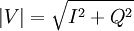
use the alpha max plus beta min algorithm. The approximation is expressed as:

For closest approximation, the use
 and
and

giving a maximum error of 3.96%.
To improve accuracy at the expense of a compare operation, if Min ≤ Max/4, we use the coefficients, α = 1 and β = 0;
otherwise, if Min > Max/4, we use α = 7/8 and β = 1/2.
Division by powers of 2 can be easily done in hardware. Error comparisons for various min/max values:

use the alpha max plus beta min algorithm. The approximation is expressed as:
For closest approximation, the use
giving a maximum error of 3.96%.
To improve accuracy at the expense of a compare operation, if Min ≤ Max/4, we use the coefficients, α = 1 and β = 0;
otherwise, if Min > Max/4, we use α = 7/8 and β = 1/2.
Division by powers of 2 can be easily done in hardware. Error comparisons for various min/max values:
 |  | Largest error (%) | Mean error (%) |
|---|---|---|---|
| 1/1 | 1/2 | 11.80 | 8.68 |
| 1/1 | 1/4 | 11.61 | 0.65 |
| 1/1 | 3/8 | 6.80 | 4.01 |
| 7/8 | 7/16 | 12.5 | 4.91 |
| 15/16 | 15/32 | 6.25 | 1.88 |
| α0 | β0 | 3.96 | 1.30 |
Sources:
- http://www.dspguru.com/book/export/html/62
- http://en.wikipedia.org/wiki/Alpha_max_plus_beta_min_algorithm
- http://www.eetimes.com/design/embedded/4007218/Digital-Signal-Processing-Tricks--High-speed-vector-magnitude-approximation/
- Mark Allie and Richard Lyons, "A Root of Less Evil," IEEE Signal Processing Magazine, March 2005, pp. 93-96.
Wednesday, June 22, 2011


Monday, June 20, 2011
Install GNOME 3 on Ubuntu 11.04
Open the terminal and run the following commands
sudo add-apt-repository ppa:gnome3-team/gnome3
sudo apt-get update
sudo apt-get dist-upgrade
sudo apt-get install gnome-shell
Thursday, June 16, 2011
Syntax Highlighting Added
Thanks to this post, I now use syntax highlighting:
http://practician.blogspot.com/2010/07/color-my-world-syntax-highlighter.html
Original code for WordPress from Alex Gorbatchev is here and description is here.
Hope you like it.
http://practician.blogspot.com/2010/07/color-my-world-syntax-highlighter.html
Original code for WordPress from Alex Gorbatchev is here and description is here.
Hope you like it.
Friday, June 10, 2011
Wednesday, June 1, 2011
Paper Review: Histograms of Oriented Gradients for Human Detection. Navneet Dalal and Bill Triggs
Thanks to Joel Andres Granados, PhD student in the IT University of Copenhagen. You saved me some effort! http://joelgranados.wordpress.com/2011/05/12/paper-histograms-of-oriented-gradients-for-human-detection/
Approach:
Approach:
- First you calculate the gradients. They tested various ways of doing this and concluded that a simple [-1,0,1] filter was best. After this calculation you will have a direction and a magnitude for each pixel.
- Divide the angle of direction in bins (Notice that you can divide 180 or 360 degrees). This is just a way to gather gradient directions into bins. A bin can be all the angles from 0 to 30 degrees.
- Divide the image in cells. Each pixel in the cell adds to a histogram of orientations based on the angle division in 2. Two really cool things to note here:
- You can avoid aliasing by interpolating votes between neighboring bins
- The magnitude of the gradient controls the way the vote is counted in the histogram
- Note that each cell is a histogram that contains the “amount” of all gradient directions in that cell.
- Create a way to group adjacent cell histograms and call it a block. For each block (group of cells) you will “normalize” it. Papers suggests something like v/sqrt(|v|^2 + e^2). Note that V is the vector representing the adjacent cell histograms of the block. Further not that || is the L-2 norm of the vector.
- Now move through the image in block steps. Each block you create is to be “normalized”. The way you move through the image allows for cells to be in more than one block (Though this is not necessary).
- For each block in the image you will get a “normalized” vector. All these vectors placed one after another is the HOG.
Comments:
- Awesome idea: The used 1239 pedestrian images. The SVM was trained with the 1239 originals and the left-right reflections. This is so cool on so many levels. Of course!! the pedestrian is still a pedestrian in the reflection image. And this little trick give double the information to the SVM with no additional storage overhead.
- They created negative training images from a data base of images which did not contain any pedestrians. Basically randomly sampled those non-pedestrian images and created the negative training set. They ran the non-pedestrian images on the resulting classifier in look for false-positives and then added these false-positives to the training set.
- A word on scale: To make detection happen they had to move a detection window through the image and run the classifier on each ROI. They did this for various scales of the image. We might not have to be so strict with this as all the flowers are going to be within a small range from the camera. Whereas pedestrians can be very close or very far from the camera. The point is that the pedestrian range is much larger.
- A margin was left in the training images. of 4 pixels.
Thursday, May 5, 2011
Simple C program that will crash any server
This is very simple C program, if executed, will defenately crash the server
Open Vi editor and type/copy the following lines
Save the file with any name, something like ... crash.c
Compile it: gcc crash.c
run it: ./a.out
And see your server crash.
Open Vi editor and type/copy the following lines
main()
{
  while(1)
  {
    fork();
  }
}
Save the file with any name, something like ... crash.c
Compile it: gcc crash.c
run it: ./a.out
And see your server crash.
Wednesday, April 27, 2011
HoG for Hand Gestures
In the Sonic Gesture project by Gijs Molinaar, hand gestures are detected by vision and converted into sound. The source code is derived from the OpenCV code by Saurabh Goyal. Link to source code is here.
Monday, April 25, 2011
Processing language comes with Image Processing Libraries
Processing is an open source programming language and environment for people who want to create images, animations, and interactions.
- Processing main page: downloads, documentation, examples.
- Integral Histogram library for Processing.
- Histogram of Oriented Gradients library for processing.
Friday, February 11, 2011
Object Detection with OpenCV - (3/3) - SVM Training
This post part 3 of a series of 3 posts at smsoft-solutions by Saurabh Goyal. To go to the original articles:
This is a follow up post to an earlier post on calculation of hog feature vectors for object detection using opencv. Here I describe how a support vector machine (svm) can be trained for a dataset containing positive and negative examples of the object to detected. The code has been commented for easier understanding of how it works :
I hope the comments were helpful to understand and use the code. To see how a large collection of files can be renamed to a sequential order which is required by this implementation refer here. Another way to read in the images of dataset could be to store the paths of all files in a text file and parse then parse the text file. I will follow up this post soon, describing how the learnt model can be used for actual detection of an object in an image.
- Object Detection Using opencv I - Integral Histogram for fast Calculation of HOG Features
- Object Detection using opencv II - Calculation of Hog Features
- Object Detection using opencv III - Training an svm for the extracted hog features
This is a follow up post to an earlier post on calculation of hog feature vectors for object detection using opencv. Here I describe how a support vector machine (svm) can be trained for a dataset containing positive and negative examples of the object to detected. The code has been commented for easier understanding of how it works :
/*This function takes in a the path and names of
64x128 pixel images, the size of the cell to be
used for calculation of hog features(which should
be 8x8 pixels, some modifications will have to be
done in the code for a different cell size, which
could be easily done once the reader understands
how the code works), a default block size of 2x2
cells has been considered and the window size
parameter should be 64x128 pixels (appropriate
modifications can be easily done for other say
64x80 pixel window size). All the training images
are expected to be stored at the same location and
the names of all the images are expected to be in
sequential order like a1.jpg, a2.jpg, a3.jpg ..
and so on or a(1).jpg, a(2).jpg, a(3).jpg ... The
explanation of all the parameters below will make
clear the usage of the function. The synopsis of
the function is as follows :

prefix : it should be the path of the images, along
with the prefix in the image name for
example if the present working directory is
/home/saurabh/hog/ and the images are in
/home/saurabh/hog/images/positive/ and are
named like pos1.jpg, pos2.jpg, pos3.jpg ....,
then the prefix parameter would be
"images/positive/pos" or if the images are
named like pos(1).jpg, pos(2).jpg,
pos(3).jpg ... instead, the prefix parameter
would be "images/positive/pos("

suffix : it is the part of the name of the image
files after the number for example for the
above examples it would be ".jpg" or ").jpg"

cell   : it should be CvSize(8,8), appropriate changes
need to be made for other cell sizes

window : it should be CvSize(64,128), appropriate
changes need to be made for other window sizes

number_samples : it should be equal to the number of
training images, for example if the
training images are pos1.jpg, pos2.jpg
..... pos1216.jpg, then it should be
1216

start_index : it should be the start index of the images'
names for example for the above case it
should be 1 or if the images were named
like pos1000.jpg, pos1001.jpg, pos1002.jpg
.... pos2216.jpg, then it should be 1000

end_index : it should be the end index of the images'
name for example for the above cases it
should be 1216 or 2216

savexml   : if you want to store the extracted features,
then you can pass to it the name of an xml
file to which they should be saved

normalization : the normalization scheme to be used for
computing the hog features, any of the
opencv schemes could be passed or -1
could be passed if no normalization is
to be done */

CvMat *train_64x128(char *prefix, char *suffix, CvSize cell,
      CvSize window, int number_samples, int start_index,
      int end_index, char *savexml = NULL, int canny = 0,
      int block = 1, int normalization = 4)
{

 char filename[50] = "\0", number[8];
 int prefix_length;
 prefix_length = strlen(prefix);
 int bins = 9;

/* A default block size of 2x2 cells is considered */

 int block_width = 2, block_height = 2;

/* Calculation of the length of a feature vector for
an image (64x128 pixels)*/

 int feature_vector_length;
 feature_vector_length = (((window.width -
       cell.width * block_width) / cell.width) +
     1) *
     (((window.height - cell.height * block_height)
       / cell.height) + 1) * 36;

/* Matrix to store the feature vectors for
all(number_samples) the training samples */

 CvMat *training = cvCreateMat(number_samples,
          feature_vector_length, CV_32FC1);

 CvMat row;
 CvMat *img_feature_vector;
 IplImage **integrals;
 int i = 0, j = 0;

 printf("Beginning to extract HoG features from
positive images\n");

 strcat(filename, prefix);

/* Loop to calculate hog features for each image one by one */

 for (i = start_index; i <= end_index; i++) {
  cvtInt(number, i);
  strcat(filename, number);
  strcat(filename, suffix);
  IplImage *img = cvLoadImage(filename);

/* Calculation of the integral histogram for
fast calculation of hog features*/

  integrals = calculateIntegralHOG(img);
  cvGetRow(training, &row, j);
  img_feature_vector
      = calculateHOG_window(integrals, cvRect(0, 0,
           window.width,
           window.height),
       normalization);
  cvCopy(img_feature_vector, &row);
  j++;
  printf("%s\n", filename);
  filename[prefix_length] = '\0';
  for (int k = 0; k < 9; k++) {
   cvReleaseImage(&integrals[k]);
  }
 }
 if (savexml != NULL) {
  cvSave(savexml, training);
 }

 return training;
}

/* This function is almost the same as
train_64x128(...), except the fact that it can
take as input images of bigger sizes and
generate multiple samples out of a single
image.

It takes 2 more parameters than
train_64x128(...), horizontal_scans and
vertical_scans to determine how many samples
are to be generated from the image. It
generates horizontal_scans x vertical_scans
number of samples. The meaning of rest of the
parameters is same.

For example for a window size of
64x128 pixels, if a 320x240 pixel image is
given input with horizontal_scans = 5 and
vertical scans = 2, then it will generate to
samples by considering windows in the image
with (x,y,width,height) as (0,0,64,128),
(64,0,64,128), (128,0,64,128), .....,
(0,112,64,128), (64,112,64,128) .....
(256,112,64,128)

The function takes non-overlapping windows
from the image except the last row and last
column, which could overlap with the second
last row or second last column. So the values
of horizontal_scans and vertical_scans passed
should be such that it is possible to perform
that many scans in a non-overlapping fashion
on the given image. For example horizontal_scans
= 5 and vertical_scans = 3 cannot be passed for
a 320x240 pixel image as that many vertical scans
are not possible for an image of height 240
pixels and window of height 128 pixels. */

CvMat *train_large(char *prefix, char *suffix,
     CvSize cell, CvSize window, int number_images,
     int horizontal_scans, int vertical_scans,
     int start_index, int end_index,
     char *savexml = NULL, int normalization = 4)
{
 char filename[50] = "\0", number[8];
 int prefix_length;
 prefix_length = strlen(prefix);
 int bins = 9;

/* A default block size of 2x2 cells is considered */

 int block_width = 2, block_height = 2;

/* Calculation of the length of a feature vector for
an image (64x128 pixels)*/

 int feature_vector_length;
 feature_vector_length = (((window.width -
       cell.width * block_width) / cell.width) +
     1) *
     (((window.height - cell.height * block_height)
       / cell.height) + 1) * 36;

/* Matrix to store the feature vectors for
all(number_samples) the training samples */

 CvMat *training = cvCreateMat(number_images
          * horizontal_scans * vertical_scans,
          feature_vector_length, CV_32FC1);

 CvMat row;
 CvMat *img_feature_vector;
 IplImage **integrals;
 int i = 0, j = 0;
 strcat(filename, prefix);

 printf("Beginning to extract HoG features
from negative images\n");

/* Loop to calculate hog features for each
image one by one */

 for (i = start_index; i <= end_index; i++) {
  cvtInt(number, i);
  strcat(filename, number);
  strcat(filename, suffix);
  IplImage *img = cvLoadImage(filename);
  integrals = calculateIntegralHOG(img);
  for (int l = 0; l < vertical_scans - 1; l++) {
   for (int k = 0; k < horizontal_scans - 1; k++) {
    cvGetRow(training, &row, j);
    img_feature_vector =
        calculateHOG_window(integrals,
       cvRect(window.width * k,
              window.height *
              l, window.width,
              window.height),
       normalization);

    cvCopy(img_feature_vector, &row);
    j++;
   }

   cvGetRow(training, &row, j);

   img_feature_vector =
       calculateHOG_window(integrals,
      cvRect(img->width -
             window.width,
             window.height * l,
             window.width,
             window.height),
      normalization);

   cvCopy(img_feature_vector, &row);
   j++;
  }

  for (int k = 0; k < horizontal_scans - 1; k++) {
   cvGetRow(training, &row, j);

   img_feature_vector =
       calculateHOG_window(integrals,
      cvRect(window.width * k,
             img->height -
             window.height,
             window.width,
             window.height),
      normalization);

   cvCopy(img_feature_vector, &row);
   j++;
  }
  cvGetRow(training, &row, j);

  img_feature_vector = calculateHOG_window(integrals,
        cvRect(img->width -
        window.width,
        img->height -
        window.height,
        window.width,
        window.height),
        normalization);

  cvCopy(img_feature_vector, &row);
  j++;

  printf("%s\n", filename);
  filename[prefix_length] = '\0';
  for (int k = 0; k < 9; k++) {
   cvReleaseImage(&integrals[k]);
  }

  cvReleaseImage(&img);

 }

 printf("%d negative samples created \n", training->rows);

 if (savexml != NULL) {
  cvSave(savexml, training);
  printf("Negative samples saved as %s\n", savexml);
 }

 return training;

}

/* This function trains a linear support vector
machine for object classification. The synopsis is
as follows :

pos_mat : pointer to CvMat containing hog feature
vectors for positive samples. This may be
NULL if the feature vectors are to be read
from an xml file

neg_mat : pointer to CvMat containing hog feature
vectors for negative samples. This may be
NULL if the feature vectors are to be read
from an xml file

savexml : The name of the xml file to which the learnt
svm model should be saved

pos_file: The name of the xml file from which feature
vectors for positive samples are to be read.
It may be NULL if feature vectors are passed
as pos_mat

neg_file: The name of the xml file from which feature
vectors for negative samples are to be read.
It may be NULL if feature vectors are passed
as neg_mat*/

void trainSVM(CvMat * pos_mat, CvMat * neg_mat, char *savexml,
       char *pos_file = NULL, char *neg_file = NULL)
{

/* Read the feature vectors for positive samples */
 if (pos_file != NULL) {
  printf("positive loading...\n");
  pos_mat = (CvMat *) cvLoad(pos_file);
  printf("positive loaded\n");
 }

/* Read the feature vectors for negative samples */
 if (neg_file != NULL) {
  neg_mat = (CvMat *) cvLoad(neg_file);
  printf("negative loaded\n");
 }

 int n_positive, n_negative;
 n_positive = pos_mat->rows;
 n_negative = neg_mat->rows;
 int feature_vector_length = pos_mat->cols;
 int total_samples;
 total_samples = n_positive + n_negative;

 CvMat *trainData = cvCreateMat(total_samples,
           feature_vector_length, CV_32FC1);

 CvMat *trainClasses = cvCreateMat(total_samples,
       1, CV_32FC1);

 CvMat trainData1, trainData2, trainClasses1, trainClasses2;

 printf("Number of positive Samples : %d\n", pos_mat->rows);

/*Copy the positive feature vectors to training
data*/

 cvGetRows(trainData, &trainData1, 0, n_positive);
 cvCopy(pos_mat, &trainData1);
 cvReleaseMat(&pos_mat);

/*Copy the negative feature vectors to training
data*/

 cvGetRows(trainData, &trainData2, n_positive, total_samples);

 cvCopy(neg_mat, &trainData2);
 cvReleaseMat(&neg_mat);

 printf("Number of negative Samples : %d\n", trainData2.rows);

/*Form the training classes for positive and
negative samples. Positive samples belong to class
1 and negative samples belong to class 2 */

 cvGetRows(trainClasses, &trainClasses1, 0, n_positive);
 cvSet(&trainClasses1, cvScalar(1));

 cvGetRows(trainClasses, &trainClasses2, n_positive, total_samples);

 cvSet(&trainClasses2, cvScalar(2));

/* Train a linear support vector machine to learn from
the training data. The parameters may played and
experimented with to see their effects*/

 CvSVM svm(trainData, trainClasses, 0, 0,
    CvSVMParams(CvSVM::C_SVC, CvSVM::LINEAR, 0, 0, 0, 2,
         0, 0, 0, cvTermCriteria(CV_TERMCRIT_EPS, 0,
            0.01)));

 printf("SVM Training Complete!!\n");

/*Save the learnt model*/

 if (savexml != NULL) {
  svm.save(savexml);
 }
 cvReleaseMat(&trainClasses);
 cvReleaseMat(&trainData);

}
I hope the comments were helpful to understand and use the code. To see how a large collection of files can be renamed to a sequential order which is required by this implementation refer here. Another way to read in the images of dataset could be to store the paths of all files in a text file and parse then parse the text file. I will follow up this post soon, describing how the learnt model can be used for actual detection of an object in an image.
Object Detection with OpenCV - (2/3) - HOG Feature Vector Calculation
This post part 2 of a series of 3 posts at smsoft-solutions by Saurabh Goyal. To go to the original articles:
This is follow up post to an earlier post where I have described how an integral histogram can be obtained from an image for fast calculation of hog features. Here I am posting the code for how this integral histogram can be used to calculate the hog feature vectors for an image window. I have commented the code for easier understanding of how it works :
I will very soon post how a support vector machine (svm) can trained using the above functions for an object using a dataset and how the learned model can be used to detect the corresponding object in an image.
- Object Detection Using opencv I - Integral Histogram for fast Calculation of HOG Features
- Object Detection using opencv II - Calculation of Hog Features
- Object Detection using opencv III - Training an svm for the extracted hog features
This is follow up post to an earlier post where I have described how an integral histogram can be obtained from an image for fast calculation of hog features. Here I am posting the code for how this integral histogram can be used to calculate the hog feature vectors for an image window. I have commented the code for easier understanding of how it works :
/* This function takes in a block as a rectangle and
calculates the hog features for the block by dividing
it into cells of size cell(the supplied parameter),
calculating the hog features for each cell using the
function calculateHOG_rect(...), concatenating the so
obtained vectors for each cell and then normalizing over
the concatenated vector to obtain the hog features for a
block */

void calculateHOG_block(CvRect block, CvMat * hog_block,
   IplImage ** integrals, CvSize cell, int normalization)
{
 int cell_start_x, cell_start_y;
 CvMat vector_cell;
 int startcol = 0;
 for (cell_start_y = block.y; cell_start_y <=
      block.y + block.height - cell.height;
      cell_start_y += cell.height) {
  for (cell_start_x = block.x; cell_start_x <=
       block.x + block.width - cell.width;
       cell_start_x += cell.width) {
   cvGetCols(hog_block, &vector_cell, startcol,
      startcol + 9);

   calculateHOG_rect(cvRect(cell_start_x,
       cell_start_y, cell.width,
       cell.height), &vector_cell,
       integrals, -1);

   startcol += 9;
  }
 }
 if (normalization != -1)
  cvNormalize(hog_block, hog_block, 1, 0, normalization);
}

/* This function takes in a window(64x128 pixels,
but can be easily modified for other window sizes)
and calculates the hog features for the window. It
can be used to calculate the feature vector for a
64x128 pixel image as well. This window/image is the
training/detection window which is used for training
or on which the final detection is done. The hog
features are computed by dividing the window into
overlapping blocks, calculating the hog vectors for
each block using calculateHOG_block(...) and
concatenating the so obtained vectors to obtain the
hog feature vector for the window*/

CvMat *calculateHOG_window(IplImage ** integrals,
      CvRect window, int normalization)
{

/*A cell size of 8x8 pixels is considered and each
block is divided into 2x2 such cells (i.e. the block
is 16x16 pixels). So a 64x128 pixels window would be
divided into 7x15 overlapping blocks*/

 int block_start_x, block_start_y, cell_width = 8;
 int cell_height = 8;
 int block_width = 2, block_height = 2;

/* The length of the feature vector for a cell is
9(since no. of bins is 9), for block it would  be
9*(no. of cells in the block) = 9*4 = 36. And the
length of the feature vector for a window would be
36*(no. of blocks in the window */

 CvMat *window_feature_vector = cvCreateMat(1,
         ((((window.width -
             cell_width * block_width)
            / cell_width) +
           1) *
          (((window.height -
             cell_height *
             block_height) /
            cell_height)
           + 1)) * 36, CV_32FC1);

 CvMat vector_block;
 int startcol = 0;
 for (block_start_y = window.y; block_start_y
      <= window.y + window.height - cell_height
      * block_height; block_start_y += cell_height) {
  for (block_start_x = window.x; block_start_x
       <= window.x + window.width - cell_width
       * block_width; block_start_x += cell_width) {
   cvGetCols(window_feature_vector, &vector_block,
      startcol, startcol + 36);

   calculateHOG_block(cvRect(block_start_x,
        block_start_y,
        cell_width * block_width,
        cell_height * block_height),
        &vector_block, integrals,
        cvSize(cell_width, cell_height),
        normalization);

   startcol += 36;
  }
 }
 return (window_feature_vector);
}
I will very soon post how a support vector machine (svm) can trained using the above functions for an object using a dataset and how the learned model can be used to detect the corresponding object in an image.
Wednesday, February 9, 2011
Object Detection with OpenCV - (1/3) - Integral Histograms
This post part 1 of a series of 3 posts at smsoft-solutions by Saurabh Goyal. To go to the original articles:
Start of borrowed stuff
Histograms of Oriented Gradients or HOG features in combination with a support vector machine have been successfully used for object Detection (most popularly pedestrian detection). An Integral Histogram representation can be used for fast calculation of Histograms of Oriented Gradients over arbitrary rectangular regions of the image. The idea of an integral histogram is analogous to that of an integral image, used by viola and jones for fast calculation of haar features for face detection. Mathematically,
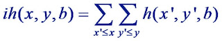
End of borrowed stuff
I will describe how the HOG features for pedestrian detection can be obtained using the above framework and how an svm can be trained for such features for pedestrian detection in a later post.
- Object Detection Using opencv I - Integral Histogram for fast Calculation of HOG Features
- Object Detection using opencv II - Calculation of Hog Features
- Object Detection using opencv III - Training an svm for the extracted hog features
Start of borrowed stuff
Histograms of Oriented Gradients or HOG features in combination with a support vector machine have been successfully used for object Detection (most popularly pedestrian detection). An Integral Histogram representation can be used for fast calculation of Histograms of Oriented Gradients over arbitrary rectangular regions of the image. The idea of an integral histogram is analogous to that of an integral image, used by viola and jones for fast calculation of haar features for face detection. Mathematically,
/*
    Function to calculate the integral histogram
*/

IplImage **calculateIntegralHOG(IplImage * in)
{

/*
   Convert the input image to grayscale
*/

 IplImage *img_gray = cvCreateImage(cvGetSize(in), IPL_DEPTH_8U, 1);
 cvCvtColor(in, img_gray, CV_BGR2GRAY);
 cvEqualizeHist(img_gray, img_gray);

/*
    Calculate the derivates of the grayscale image in the x and y directions using a
    sobel operator and obtain 2 gradient images for the x and y directions
*/

 IplImage *xsobel, *ysobel;
 xsobel = doSobel(img_gray, 1, 0, 3);
 ysobel = doSobel(img_gray, 0, 1, 3);
 cvReleaseImage(&img_gray);

/*
    Create an array of 9 images (9 because I assume bin size 20 degrees and unsigned gradient
    ( 180/20 = 9), one for each bin which will have zeroes for all pixels, except for the
    pixels in the original image for which the gradient values correspond to the particular
    bin. These will be referred to as bin images. These bin images will be then used to
    calculate the integral histogram, which will quicken the calculation of HOG descriptors
*/

 IplImage **bins = (IplImage **) malloc(9 * sizeof(IplImage *));
 for (int i = 0; i < 9; i++) {
  bins[i] = cvCreateImage(cvGetSize(in), IPL_DEPTH_32F, 1);
  cvSetZero(bins[i]);
 }

/*
    Create an array of 9 images ( note the dimensions of the image, the cvIntegral() function
    requires the size to be that), to store the integral images calculated from the above bin
    images. These 9 integral images together constitute the integral histogram
*/

 IplImage **integrals = (IplImage **) malloc(9 * sizeof(IplImage *));
 for (int i = 0; i < 9; i++) {
  integrals[i] =
      cvCreateImage(cvSize(in->width + 1, in->height + 1),
      IPL_DEPTH_64F, 1);
 }

/*
    Calculate the bin images. The magnitude and orientation of the gradient at each pixel
    is calculated using the xsobel and ysobel images.
    {Magnitude = sqrt(sq(xsobel) + sq(ysobel) ), gradient = itan (ysobel/xsobel) }.
    Then according to the orientation of the gradient, the value of the corresponding pixel
    in the corresponding image is set
*/

 int x, y;
 float temp_gradient, temp_magnitude;
 for (y = 0; y < in->height; y++) {

/*
     ptr1 and ptr2 point to beginning of the current row in the xsobel and ysobel images
     respectively. ptrs[i] point to the beginning of the current rows in the bin images
*/

  float *ptr1 =
      (float *)(xsobel->imageData + y * (xsobel->widthStep));
  float *ptr2 =
      (float *)(ysobel->imageData + y * (ysobel->widthStep));
  float **ptrs = (float **)malloc(9 * sizeof(float *));
  for (int i = 0; i < 9; i++) {
   ptrs[i] =
       (float *)(bins[i]->imageData +
          y * (bins[i]->widthStep));
  }

/*
    For every pixel in a row gradient orientation and magnitude are calculated
    and corresponding values set for the bin images.
*/

  for (x = 0; x < in->width; x++) {

/*
    If the xsobel derivative is zero for a pixel, a small value is added to it, to avoid
    division by zero. atan returns values in radians, which on being converted to degrees,
    correspond to values between -90 and 90 degrees. 90 is added to each orientation, to
    shift the orientation values range from {-90-90} to {0-180}. This is just a matter of
    convention. {-90-90} values can also be used for the calculation.
*/

   if (ptr1[x] == 0) {
    temp_gradient =
        ((atan(ptr2[x] / (ptr1[x] + 0.00001))) *
         (180 / PI)) + 90;
   } else {
    temp_gradient =
        ((atan(ptr2[x] / ptr1[x])) * (180 / PI)) +
        90;
   }
   temp_magnitude =
       sqrt((ptr1[x] * ptr1[x]) + (ptr2[x] * ptr2[x]));

/*
    The bin image is selected according to the gradient values. The corresponding pixel
    value is made equal to the gradient magnitude at that pixel in the corresponding bin image
*/

   if (temp_gradient <= 20) {
    ptrs[0][x] = temp_magnitude;
   } else if (temp_gradient <= 40) {
    ptrs[1][x] = temp_magnitude;
   } else if (temp_gradient <= 60) {
    ptrs[2][x] = temp_magnitude;
   } else if (temp_gradient <= 80) {
    ptrs[3][x] = temp_magnitude;
   } else if (temp_gradient <= 100) {
    ptrs[4][x] = temp_magnitude;
   } else if (temp_gradient <= 120) {
    ptrs[5][x] = temp_magnitude;
   } else if (temp_gradient <= 140) {
    ptrs[6][x] = temp_magnitude;
   } else if (temp_gradient <= 160) {
    ptrs[7][x] = temp_magnitude;
   } else {
    ptrs[8][x] = temp_magnitude;
   }
  }
 }

 cvReleaseImage(&xsobel);
 cvReleaseImage(&ysobel);

/*Integral images for each of the bin images are calculated*/

 for (int i = 0; i < 9; i++) {
  cvIntegral(bins[i], integrals[i]);
 }

 for (int i = 0; i < 9; i++) {
  cvReleaseImage(&bins[i]);
 }

/*
    The function returns an array of 9 images which consitute the integral histogram
*/

 return (integrals);

}
The following demonstrates how the integral histogram calculated using the above function can be used to calculate the histogram of oriented gradients for any rectangular region in the image: /*
The following function takes as input the rectangular cell for which the histogram of
oriented gradients has to be calculated, a matrix hog_cell of dimensions 1x9 to store
the bin values for the histogram, the integral histogram, and the normalization scheme
to be used. No normalization is done if normalization = -1
*/
void calculateHOG_rect(CvRect cell, CvMat * hog_cell,
IplImage ** integrals, int normalization)
{
/* Calculate the bin values for each of the bin of the histogram one by one */
for (int i = 0; i < 9; i++) {
float a = ((double *)(integrals[i]->imageData + (cell.y)
* (integrals[i]->widthStep)))[cell.x];
float b =
((double *)(integrals[i]->imageData + (cell.y + cell.height)
* (integrals[i]->widthStep)))[cell.x +
cell.width];
float c = ((double *)(integrals[i]->imageData + (cell.y)
* (integrals[i]->widthStep)))[cell.x +
cell.width];
float d =
((double *)(integrals[i]->imageData + (cell.y + cell.height)
* (integrals[i]->widthStep)))[cell.x];
((float *)hog_cell->data.fl)[i] = (a + b) - (c + d);
}
/*
Normalize the matrix
*/
if (normalization != -1) {
cvNormalize(hog_cell, hog_cell, 1, 0, normalization);
}
}
End of borrowed stuff
I will describe how the HOG features for pedestrian detection can be obtained using the above framework and how an svm can be trained for such features for pedestrian detection in a later post.

Subscribe to:
Posts (Atom)